A Vlookup Tutorial Part One - Getting the Formula Right

Vlookup is one of those functions in Excel that is so useful when people get it to work correctly. The problem is people are sometimes overwhelmed when they see the final outcome in the formula bar. This post will show you step-by-step on how to use Vlookup. Part 2 will use the same data but will take vlookup to the next level by using 2 separate files. It will also use the 'If Statement' and 'IsNA function' as an error-handling technique on how to stop the dreaded #N/A's.

For simplicity reasons, we will use one file with two worksheets. First, start with a new file and call it "Vlookup Tutorial". You'll notice the default parameters of a new workbook includes 3 worksheets: Sheet1, Sheet2 and Sheet3. Right-click directly on top of the name of Sheet3 and select 'Delete'. Rename Sheet1 to 'Data'. Rename Sheet2 to 'Reports'. Your file should now look like Figure 1.1.

Figure 1.1























Under the 'Data' Worksheet, enter Student in A1 and Score in A2. Enter the following names under Student: Joe Smith, John Doe, Larry Wang, Alicia Sloan, and Mary Jones. Enter the following under Score: 66, 88, 55, 98 and 90. Do some crazy formatting like adjusting the column widths, left alignment, removing gridlines, adding borders and adding color. The 'Data' worksheet should now look like Figure 1.2.

Figure 1.2
















Now copy all cells from A1 to B6 and paste them into A1 of the 'Reports' worksheet. Clear all the scores for the 'Reports' worksheet. Adjust the columns. Remove the gridlines (Don't know how? Click here). The 'Reports' worksheet should now look like Figure 1.3.

Figure 1.3
















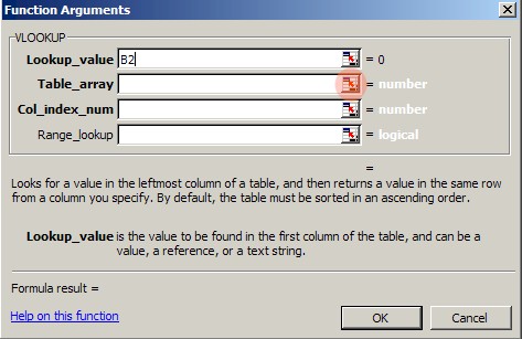
Before beginning the Vlookup function, click once on cell B2 of the 'Reports' worksheet. To start the Vlookup you'll notice there is a function symbol you need to click on. It looks like fx and is right beside the formula bar. See Figure 1.4 if you can't find it.

Figure 1.4
















After you click on the function symbol (fx), a new window will pop up asking you which function you wish to use. From the category drop-down box, select 'Lookup & Reference' and scroll down until you see Vlookup. Highlight Vlookup and press the OK button. See Figure 1.5.

Figure 1.5
















After pressing the OK button, the window changes to Function Arguments. There are 4 arguments to enter. We'll start with the first argument, the Lookup_value. You'll notice beside each argument there is a place to enter manually. Just beside that is a Search Symbol. It looks like a little square box with a red arrow inside of it. See Figure 1.6.

Figure 1.6













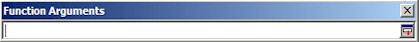
Now click on the Search button as shown on in Figure 1.6. After clicking this button, you'll notice the windows shrinks into one thin window. See Figure 1.7.

Figure 1.7


Excel now wants to know where the Lookup_value should come from. If you're not already there, go to the 'Reports' worksheet by clicking on the name near the bottom of the worksheet. Click on the cell A2. The function argument should now look like Figure 1.8.

Figure 1.8

Now, click on the Search Button. You should now be back to the main Function Arguments window with A2 as the parameter for the first argument, Vlookup_value. See Figure 1.9.

Figure 1.9

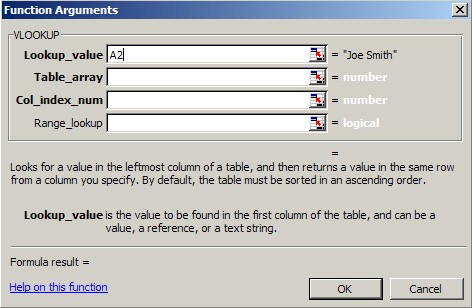
For the second argument, Table_array, click it's according Search Button. See Figure 2.0.

Figure 2.0

Like the first argument, when you press the Table_array Search button, the window shrinks to a sliver-like appearance. This time, click on the name of the 'Data' worksheet which is located near the bottom left corner of the screen. See Figure 2.1.

Figure 2.1

Highlight area A2 to B6. Leave the area highlighted and then press the Search button once again. You should now be back to the main Function Arguments window. It should look like Figure 2.2.

Figure 2.2

Now, the Table_array data should now show Data!A2:B6. Change it to the following:

Data!$A$2:$B$6

Why? By adding the dollar signs between the selected range, the range will now stay the same even if you copy and paste the formula somewhere else. See Figure 2.3.

(Editor's Note: There is another way of adding dollar signs quickly. If you click between A2 and press F4(the function key on your keyboard), A2 will change to $A$2 automatically. Accordingly, by pressing the F4 key when the cursor is placed in between B6, it will change B6 to $B$6.)

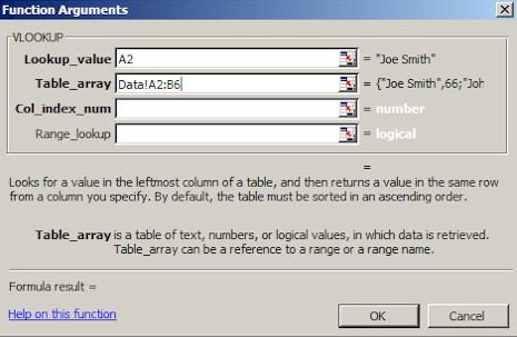
Figure 2.3

Now, for the third argument, the Col_index_num, enter the number 2. This tells the Vlookup function to return the value of the cell in the second column which is the Score Column in the 'Data' worksheet.

For the fourth and final argument, enter the word 'false'. This argument should always be false. If anyone out there knows why this argument would ever be 'true', leave a comment so I can learn from you. You can look at Figure 2.4 to make sure everything looks correct. Now that all the arguments are complete, you can press the OK button.

Figure 2.4

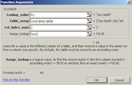
After pressing the OK button, the 'Reports' worksheet should now have the number 66 in cell B2. Copy B2 and paste it from B2 to B6. The file should now look complete.

To download the completed file click here.

That's it. Keep Excelling!