This tutorial will take Vlookup to the next level by using two files while using 'If Statements' and 'IsNA' functions for error handling. If you have not already done so, it would easier to follow this tutorial by going through part one first. Click here to go to part one. This tutorial is a continuation of part one. Therefore, you can use the file from part one for this tutorial by clicking here. We will be running through this tutorial a little faster than part one as we assume you are beginning to understand some of the basics of Excel and are moving closer to the intermediate level.
Okay, let's first start with splitting the file from part one into two files. Open the Vlookup Tutorial from part one. You will remember that this file has 2 worksheets: 'Data' and 'Reports'.
Right-click directly over the name of the 'Data' worksheet and select 'Move or Copy...'. From the 'To book' drop-down box, select '(new book)' and press the OK button. The new book should be called 'Book1' if you haven't been using Excel today. Rename the file to 'Data For Vlookup'. The new file, Data for Vlookup, should now only contain one worksheet called 'Data'.
Go back to the original file, Vlookup Tutorial Part One, and rename it to 'Reports For Vlookup'. The renamed file, Reports for Vlookup, should now only contain one worksheet called 'Reports'.
Now we are going to look at the vlookup formula a little closer. On the newly renamed file, 'Reports For Vlookup', click on cell B2. The contents of this cell has changed to reflect the movement of the data to the 'Data For Vlookup' file. See Figure 1.1.
Figure 1.1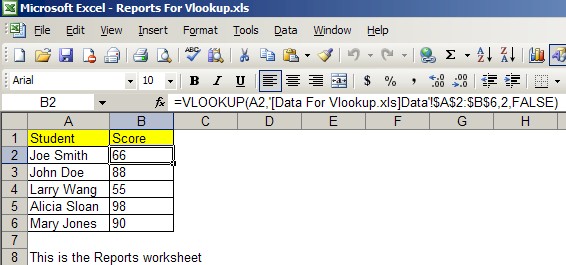
The formula bar is starting to look a little crazy. Let's break it down. From Figure 1.1 formula bar we see:
=VLOOKUP(A2,'[Data For Vlookup.xls]Data'!$A$2:$B$6,2,FALSE)
where
A2 is the first argument, Lookup_value. This is the value you want to find and match from another file or worksheet.
'[Data For Vlookup.xls]Data'!$A$2:$B$6 is the second argument. This is the Table_array. This is the area where you will search for a match from the Lookup_value. It can be another worksheet in the same or different file.
2 is the third argument. This is the Column_index_num. It asks us what column number to search for the Lookup_value in the Table_array.
FALSE is the fourth argument. This is the Range_lookup. I would always keep this as FALSE.
With all of this to absorb, let's move on to Error Handling.
There are many types of errors you can get such as #REF and #N/A. For example, If you enter a Column_index_num of 3 for the third argument, you will get a #REF error because there isn't a third column in the Table_array in our 'Data' worksheet. If Vlookup can't find a match for the Lookup_value in the Table_array you will get a #N/A error. Let's try it out. Go to the 'Reports for Vlookup' file and change the value of cell A2, Joe Smith, to John Smith. See Figure 1.2.
Figure 1.2
You will see from Figure 1.2 that cell B2 shows a #N/A error. Let's change the formula in cell B2. Currently, the formula in cell B2 looks like this:
=VLOOKUP(A2,'[Data For Vlookup.xls]Data'!$A$2:$B$6,2,FALSE)
I want you to first remove the equals sign (=) and then CUT (not COPY) the rest of the data to your clipboard. After you remove the equals sign, CUT the rest of the data by first left-clicking in the formula bar once. To do this, press CTRL and A on your keyboard at the same time. This will SELECT ALL the data in the formula bar. Finally, press CTRL and X on your keyboard at the same time. This will CUT the data in the formula bar to your clipboard. If done correctly, cell B2 should now be empty.
Now let's step-by-step add an 'If Statement' and an 'ISNA' into the formula.
First enter the following into cell B2:
=if(isna(
Now, press Ctrl and V at the same time to paste the Vlookup formula from the clipboard. Your formula should now look like this:
=if(isna(VLOOKUP(A2,'[Data For Vlookup.xls]Data'!$A$2:$B$6,2,FALSE)
Add a little bit more to the end of this formula as shown in red:
=if(isna(VLOOKUP(A2,'[Data For Vlookup.xls]Data'!$A$2:$B$6,2,FALSE)),"Student not found.",
Now, press Ctrl and V at the same time to paste the Vlookup formula from the clipboard again. Your formula should now look like this:
=if(isna(VLOOKUP(A2,'[Data For Vlookup.xls]Data'!$A$2:$B$6,2,FALSE)),"Student not found.",VLOOKUP(A2,'[Data For Vlookup.xls]Data'!$A$2:$B$6,2,FALSE)
Now, just add one more closing bracket for the 'If Statement'. Your formula should now look like this:
=if(isna(VLOOKUP(A2,'[Data For Vlookup.xls]Data'!$A$2:$B$6,2,FALSE)),"Student not found.",VLOOKUP(A2,'[Data For Vlookup.xls]Data'!$A$2:$B$6,2,FALSE))
Press Enter on your keyboard to complete the formula. If done correctly, cell B2 should look like Figure 1.3.
Figure 1.3
Adjust column B2 so the text 'Student not found.' fits properly. Copy cell B2 and paste it down to B6. You're done! Let's go back and review the complete formula in cell B2 first.
=if(isna(VLOOKUP(A2,'[Data For Vlookup.xls]Data'!$A$2:$B$6,2,FALSE)),"Student not found.",VLOOKUP(A2,'[Data For Vlookup.xls]Data'!$A$2:$B$6,2,FALSE))
The blue area is the logical test for the 'If Statement'. In normal wording, it tells Excel, "If the Vlookup I'm using results in a #N/A error, then to go to the TRUE part of the 'If Statement'.
The red area is what occurs if the logical test in the blue area is TRUE.
The green area is what occurs if the logical test in the blue area is FALSE.
Let's see an example of the 'If Statement' in a clear example.
=if(A2="Joe Smith","66","Student not found.")
Here you can see if cell A2 equals 'Joe Smith', then let B2 equal to '66'. If A2 doesn't equal 'Joe Smith', then let B2 equal to 'Student not found.'.
To download the completed files click here.
That's it! Keep Excelling!
No comments:
Post a Comment