Conditional Formatting is a very simple, yet useful tool in data analysis. By understanding how it works, you can cut down your time tracking data entry errors by allowing you to visually see if specific criteria was met or not. The Countif formula gives you the total of the number of times a condition has been met. Let's get started with a simple example by downloading the file from Figure 1.1 by clicking here.
See Figure 1.1
From Figure 1.1, we want to see which of the 20 students have a failing grade. Highlight cells B2:B21 and then select Format>Conditional Formatting... See Figure 1.2.
Figure 1.2
After you left click on 'Conditional Formatting...', a Conditional Formatting popup box should be displayed. See Figure 1.3.
Figure 1.3
Change the values in the Conditional Formatting popup box to the following as shown in Figure 1.4. (i.e. Cell Valus Is less than 50)
Figure 1.4
Now, click on the 'Format...' button on the far right. See Figure 1.5
Figure 1.5
After you click on the 'Format...' button, a 'Format Cells' popup menu is displayed. Select the 'Pattern' tab at the top of the menu. Select the Yellow box in the color palette. Pres the OK button. See Figure 1.6.
Figure 1.6
Now, the Course Mark cell color should be yellow for Joe Blow, Stanley Berdych, Bill Doughnut and Peter Griffin. See Figure 1.7.
Figure 1.7
Now, in cell A23 enter "Total Marks under 50". In cell B23 enter the following formula:
=COUNTIF(B2:B21,"<50")
where
COUNTIF is the formula
B2:B21 is the range
"<50" is the criteria
which in plain English tells us to look at the course marks of the students from cells B2 to B21 and count how many cells are less than a course mark of 50. See Figure 1.8.
Figure 1.8
If you examined the figures carefully, you will see conditional formatting did not catch a data entry error: Lester Judd's score of 20 should be yellow and there should be 5 marks under 50! The problem is Lester's mark of 20 was entered as the number 2 and the letter O (instead of the number zero). This will be handled in a different tutorial: Data Validation.
For the completed file, click here.
That's it. Keep Excelling!
Conditional Formatting and the Countif Formula
How to Find Column A
There are times in the workplace when employees 'accidently' hide columns or rows in Excel and they start to panic and say, " Where did my data go? I spent all day entering these numbers and I can't find it. I hope I didn't delete anything! " Well, sometimes the person did delete the data and you can only pray that they saved a backup copy. Some other times, they might have just 'hidden' the data by mistake. Let's take a look at the latter situation.
Figure 1.1
First, check to see if the panes have been frozen. If they are, we'll turn it off by going to Windows>Unfreeze Panes. See Figure 1.2.
Figure 1.2
Now, type A1 into the Name Box and press the Enter key. See Figure 1.3.
Figure 1.3
Now go to Format>Column>Unhide. See Figure 1.4.
Figure 1.4
You should now be able to see Column A (and myself). See Figure 1.5
Figure 1.5
That's it! Keep Excelling!
Uppercase Everything in Excel
This simple tutorial will show you how to change everything in a worksheet to uppercase.
To begin, click here to download the file as shown in Figure 1.1.
Figure 1.1
Right-click cell A1 of the worksheet named 'All Cases' and select 'Copy'. Now, go to the other worksheet by clicking on the name 'Convert To Uppercase'. See Figure 1.2 if you can't find the name.
Figure 1.2
Now that you're on the proper spreadsheet, right-click cell A1 of the 'Convert To Uppercase' worksheet and select Paste Special. After clicking Paste Special, a new window will pop up called 'Paste Special'. Near the bottom left-hand corner of the 'Paste Special' window, click on Paste Link. See Figure 1.3.
Figure 1.3
After pressing 'Paste Link', the 'Paste Special' window will close automatically. Your 'Convert To Uppercase' worksheet should now look like Figure 1.4.
Figure 1.4
Notice that the value of cell A1 is equal to A1 of the 'All Cases' worksheet. Take a closer look at the formula bar of cell A1 on the 'Convert To Uppercase' worksheet and you should see the following:
='All Cases'!$A$1
Remove the dollar($) signs so the formula of cell A1 looks like:
='All Cases'!A1
Now, change the formula by adding the UPPER function. The formula should now look like:
=UPPER('All Cases'!A1)
Copy the above formula and paste it from A1 to C11. Your worksheet should now look like Figure 1.5.
Figure 1.5
To keep the formatting the same as the 'All Cases' worksheet, go back to the 'All Cases' worksheet and right-click the top left corner of the worksheet and select 'Copy'. See Figure 1.6 if you aren't sure where the top left corner is.
Figure 1.6
Go back to the 'Convert To Uppercase' worksheet and right-click the top left corner of the worksheet and select 'Paste Special'. The 'Paste Special' window will appear. Click on the 'Formats' option button and press the OK button. See Figure 1.7.
Figure 1.7
After pressing the OK button, the 'Paste Special' window should disappear and the formats for both worksheets should now be the same. Finally, remove the gridlines.
(Editors Note: If you would like to remove the formulas and keep the values, right-click the upper left corner of the 'Convert to Uppercase' worksheet and select Copy. Right-click the upper left corner again and select Paste Special. Select 'Values' and press the OK button.)
To download the completed file (formulas are intact) click here.
That's it! Keep Excelling!
A Vlookup Tutorial Part Two - Using Two Files With Error Handling
This tutorial will take Vlookup to the next level by using two files while using 'If Statements' and 'IsNA' functions for error handling. If you have not already done so, it would easier to follow this tutorial by going through part one first. Click here to go to part one. This tutorial is a continuation of part one. Therefore, you can use the file from part one for this tutorial by clicking here. We will be running through this tutorial a little faster than part one as we assume you are beginning to understand some of the basics of Excel and are moving closer to the intermediate level.
Okay, let's first start with splitting the file from part one into two files. Open the Vlookup Tutorial from part one. You will remember that this file has 2 worksheets: 'Data' and 'Reports'.
Right-click directly over the name of the 'Data' worksheet and select 'Move or Copy...'. From the 'To book' drop-down box, select '(new book)' and press the OK button. The new book should be called 'Book1' if you haven't been using Excel today. Rename the file to 'Data For Vlookup'. The new file, Data for Vlookup, should now only contain one worksheet called 'Data'.
Go back to the original file, Vlookup Tutorial Part One, and rename it to 'Reports For Vlookup'. The renamed file, Reports for Vlookup, should now only contain one worksheet called 'Reports'.
Now we are going to look at the vlookup formula a little closer. On the newly renamed file, 'Reports For Vlookup', click on cell B2. The contents of this cell has changed to reflect the movement of the data to the 'Data For Vlookup' file. See Figure 1.1.
Figure 1.1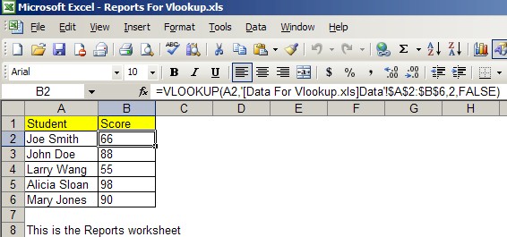
The formula bar is starting to look a little crazy. Let's break it down. From Figure 1.1 formula bar we see:
=VLOOKUP(A2,'[Data For Vlookup.xls]Data'!$A$2:$B$6,2,FALSE)
where
A2 is the first argument, Lookup_value. This is the value you want to find and match from another file or worksheet.
'[Data For Vlookup.xls]Data'!$A$2:$B$6 is the second argument. This is the Table_array. This is the area where you will search for a match from the Lookup_value. It can be another worksheet in the same or different file.
2 is the third argument. This is the Column_index_num. It asks us what column number to search for the Lookup_value in the Table_array.
FALSE is the fourth argument. This is the Range_lookup. I would always keep this as FALSE.
With all of this to absorb, let's move on to Error Handling.
There are many types of errors you can get such as #REF and #N/A. For example, If you enter a Column_index_num of 3 for the third argument, you will get a #REF error because there isn't a third column in the Table_array in our 'Data' worksheet. If Vlookup can't find a match for the Lookup_value in the Table_array you will get a #N/A error. Let's try it out. Go to the 'Reports for Vlookup' file and change the value of cell A2, Joe Smith, to John Smith. See Figure 1.2.
Figure 1.2
You will see from Figure 1.2 that cell B2 shows a #N/A error. Let's change the formula in cell B2. Currently, the formula in cell B2 looks like this:
=VLOOKUP(A2,'[Data For Vlookup.xls]Data'!$A$2:$B$6,2,FALSE)
I want you to first remove the equals sign (=) and then CUT (not COPY) the rest of the data to your clipboard. After you remove the equals sign, CUT the rest of the data by first left-clicking in the formula bar once. To do this, press CTRL and A on your keyboard at the same time. This will SELECT ALL the data in the formula bar. Finally, press CTRL and X on your keyboard at the same time. This will CUT the data in the formula bar to your clipboard. If done correctly, cell B2 should now be empty.
Now let's step-by-step add an 'If Statement' and an 'ISNA' into the formula.
First enter the following into cell B2:
=if(isna(
Now, press Ctrl and V at the same time to paste the Vlookup formula from the clipboard. Your formula should now look like this:
=if(isna(VLOOKUP(A2,'[Data For Vlookup.xls]Data'!$A$2:$B$6,2,FALSE)
Add a little bit more to the end of this formula as shown in red:
=if(isna(VLOOKUP(A2,'[Data For Vlookup.xls]Data'!$A$2:$B$6,2,FALSE)),"Student not found.",
Now, press Ctrl and V at the same time to paste the Vlookup formula from the clipboard again. Your formula should now look like this:
=if(isna(VLOOKUP(A2,'[Data For Vlookup.xls]Data'!$A$2:$B$6,2,FALSE)),"Student not found.",VLOOKUP(A2,'[Data For Vlookup.xls]Data'!$A$2:$B$6,2,FALSE)
Now, just add one more closing bracket for the 'If Statement'. Your formula should now look like this:
=if(isna(VLOOKUP(A2,'[Data For Vlookup.xls]Data'!$A$2:$B$6,2,FALSE)),"Student not found.",VLOOKUP(A2,'[Data For Vlookup.xls]Data'!$A$2:$B$6,2,FALSE))
Press Enter on your keyboard to complete the formula. If done correctly, cell B2 should look like Figure 1.3.
Figure 1.3
Adjust column B2 so the text 'Student not found.' fits properly. Copy cell B2 and paste it down to B6. You're done! Let's go back and review the complete formula in cell B2 first.
=if(isna(VLOOKUP(A2,'[Data For Vlookup.xls]Data'!$A$2:$B$6,2,FALSE)),"Student not found.",VLOOKUP(A2,'[Data For Vlookup.xls]Data'!$A$2:$B$6,2,FALSE))
The blue area is the logical test for the 'If Statement'. In normal wording, it tells Excel, "If the Vlookup I'm using results in a #N/A error, then to go to the TRUE part of the 'If Statement'.
The red area is what occurs if the logical test in the blue area is TRUE.
The green area is what occurs if the logical test in the blue area is FALSE.
Let's see an example of the 'If Statement' in a clear example.
=if(A2="Joe Smith","66","Student not found.")
Here you can see if cell A2 equals 'Joe Smith', then let B2 equal to '66'. If A2 doesn't equal 'Joe Smith', then let B2 equal to 'Student not found.'.
To download the completed files click here.
That's it! Keep Excelling!
A Vlookup Tutorial Part One - Getting the Formula Right
Vlookup is one of those functions in Excel that is so useful when people get it to work correctly. The problem is people are sometimes overwhelmed when they see the final outcome in the formula bar. This post will show you step-by-step on how to use Vlookup. Part 2 will use the same data but will take vlookup to the next level by using 2 separate files. It will also use the 'If Statement' and 'IsNA function' as an error-handling technique on how to stop the dreaded #N/A's.
For simplicity reasons, we will use one file with two worksheets. First, start with a new file and call it "Vlookup Tutorial". You'll notice the default parameters of a new workbook includes 3 worksheets: Sheet1, Sheet2 and Sheet3. Right-click directly on top of the name of Sheet3 and select 'Delete'. Rename Sheet1 to 'Data'. Rename Sheet2 to 'Reports'. Your file should now look like Figure 1.1.
Figure 1.1
Under the 'Data' Worksheet, enter Student in A1 and Score in A2. Enter the following names under Student: Joe Smith, John Doe, Larry Wang, Alicia Sloan, and Mary Jones. Enter the following under Score: 66, 88, 55, 98 and 90. Do some crazy formatting like adjusting the column widths, left alignment, removing gridlines, adding borders and adding color. The 'Data' worksheet should now look like Figure 1.2.
Figure 1.2
Now copy all cells from A1 to B6 and paste them into A1 of the 'Reports' worksheet. Clear all the scores for the 'Reports' worksheet. Adjust the columns. Remove the gridlines (Don't know how? Click here). The 'Reports' worksheet should now look like Figure 1.3.
Figure 1.3
Before beginning the Vlookup function, click once on cell B2 of the 'Reports' worksheet. To start the Vlookup you'll notice there is a function symbol you need to click on. It looks like fx and is right beside the formula bar. See Figure 1.4 if you can't find it.
Figure 1.4
After you click on the function symbol (fx), a new window will pop up asking you which function you wish to use. From the category drop-down box, select 'Lookup & Reference' and scroll down until you see Vlookup. Highlight Vlookup and press the OK button. See Figure 1.5.
Figure 1.5
After pressing the OK button, the window changes to Function Arguments. There are 4 arguments to enter. We'll start with the first argument, the Lookup_value. You'll notice beside each argument there is a place to enter manually. Just beside that is a Search Symbol. It looks like a little square box with a red arrow inside of it. See Figure 1.6.
Figure 1.6
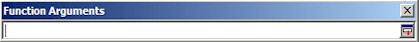
Now click on the Search button as shown on in Figure 1.6. After clicking this button, you'll notice the windows shrinks into one thin window. See Figure 1.7.
Figure 1.7
Excel now wants to know where the Lookup_value should come from. If you're not already there, go to the 'Reports' worksheet by clicking on the name near the bottom of the worksheet. Click on the cell A2. The function argument should now look like Figure 1.8.
Figure 1.8

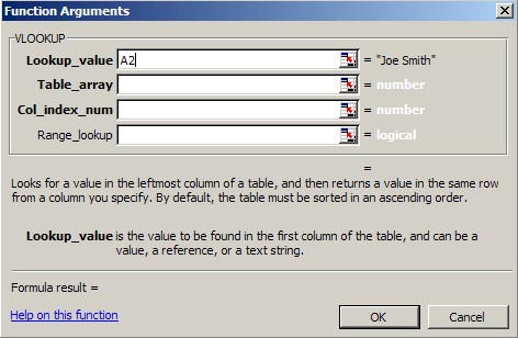
Figure 2.0


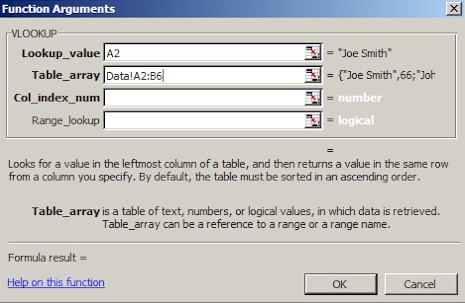
Figure 2.3

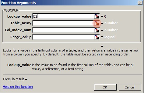
Now, for the third argument, the Col_index_num, enter the number 2. This tells the Vlookup function to return the value of the cell in the second column which is the Score Column in the 'Data' worksheet.
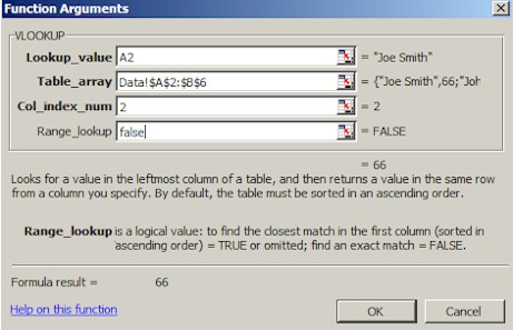
After pressing the OK button, the 'Reports' worksheet should now have the number 66 in cell B2. Copy B2 and paste it from B2 to B6. The file should now look complete.
The Power of AutoFilters and Subtotals
AutoFilter is a powerful feature where data can be filtered anyway you want. Subtotal works in conjunction with AutoFilter to display totals only in the filtered data. For example, if you wanted to know the total cost of Product A in the Northwest Region of the company, you can do it with AutoFilter and Subtotal. To get started, let's work first with AutoFilter and a simple spreadsheet.

Highlight the area as shown in Figure 1.2.


You will notice that you only see rows 1 to 4 visibile. You will also notice that the row numbers changed to the colour blue to tell you the user that there is at least one filter on. To turn off all filters go to the menu Data>Filter>Show All. This will remove all filters. The first row that is not part of the filter is row 12. This is very important for Subtotals. If you enter data into row 12 then the Autofilter will view row 12 as a part of the filter and you will not see the subtotal.


How Do You Remove Gridlines?
Go to Tools>Options>View and remove the check for Gridlines. Now your spreadsheet will look like a blank white page. I hate gridlines.
Should you upgrade to Excel 2007?
I always wondered when the 65,536 row limit would be extended for Excel. Now it's ridiculous. Take a look. I'm only going to show the major points here. To see all, visit http://www.mvps.org/visio/Excel_2007.htm.
The total number of available columns in Excel
Old - 256
New - 16000+
The total number of available rows in Excel
Old - 64,000+
New - 1,000,000+
Total amount of PC memory that Excel can use
Old - 1GB
New - Maximum allowed by Windows
Unique Colours Per Workbook
Old - 56
New - 4.3 billion
Number of conditional format conditions on a cell
Old - 3 conditions
New - Limited by available memory
Number of levels of sorting on a range or table
Old - 3
New - 64
Number of items shown in the Auto-Filter dropdown
Old - 1,000
New - 10,000
The total number of characters that can display in a cell
Old - 1k (when the text is formatted)
New - 32k or as many as will fit in the cell (regardless of formatting)
The maximum length of formulas (in characters)
Old - 1k characters
New - 8k characters
The number of levels of nesting that Excel allows in formulas
Old - 7
New - 64
Maximum number of arguments to a function
Old - 30
New - 255
Number of rows allowed in a Pivot Table
Old - 64k
New - 1M
Number of columns allowed in a Pivot Table
Old - 255
New - 16k
Maximum number of unique items within a single Pivot Field
Old - 32k
New - 1M
The number of fields (as seen in the field list) that a single PivotTable can have
Old - 255
New - 16k
A resizeable formula bar
The Name Manager helps organize, update and manage multiple name ranges from a central location.
If you hover over the different table formats in the Table Gallery, you will see a live preview of how your table will look. Some of the formats include alternating colours for rows (usually light and dark). If you delete a row, Excel 2007 will maintain the alternating pattern.
Functions
Yes there are more functions. There are 343 functions with 51 new functions.
CUBERANKEDMEMBER
Returns the nth, or ranked, member in a set. Use to return one or more elements in a set, such as the top sales performer or top 10 students.
Cube
CONVERT
Converts a number from one measurement system to another
Engineering
DELTA
Tests whether two values are equal
SQL.REQUEST
Connects with an external data source and runs a query from a worksheet, then returns the result as an array without the need for macro programming.
Acrobat files
Excel 2007 spreadsheets will also be able to export to PDF. A special PDF writer will no longer be required.